Closure-Compatible Resonance

Abstract

Many physical systems exhibit strong stability constraints and apparent stochasticity that are typically described in terms of force-driven dynamics, dissipation, and suppression of instabilities. This paper proposes a complementary viewpoint: persistence, confinement, and controllability are governed primarily by closure-compatible resonant configurations – admissible structures whose internal phase evolution remains bounded and self-consistent. Within this perspective, “matter” is interpreted as the set of dynamically persistent closure classes, while “forces” emerge as effective tendencies when a system is displaced into inadmissible regions of configuration space.

We formalize this idea by introducing closure deficit functionals \(C\) that quantify departure from closure compatibility. A closure penalty induces an effective potential \(V(C)\) with a stable minimum at closure; the generic leading-order behavior near admissibility is quadratic, \(V \approx \kappa C^2\), yielding admissibility gradients \(\mathbf{F}_{\mathrm{AG}}=-\nabla V\). Two explicit deficit constructions are presented: (A) a lattice-distance deficit in phase-increment space, producing quantized resonance basins and basin boundaries; and (B) a geometric mismatch deficit in rendered space, providing an intuitive closure error tied to observable geometry.

To complement the theory with operational evidence, we define entrainment closure on the event-phase circle \(S^1\) using phase-locking value (PLV) and the operational closure deficit \(C_{\text{phase}}=1-\mathrm{PLV}\). PLV is a standard synchronization measure used across applied dynamical systems and signal analysis [1]. We implement this definition in a minimal intermittent “plasmoid reconnection entrainment” proxy simulation whose drive can act as threshold modulation (gating), parametric modulation, or additive forcing. Sweeps over drive amplitude \(A\) and detuning ratio \(f_d/f_0\) show: (i) a minimum drive authority is required for strong phase closure, producing Arnold-tongue–like locking regions; and (ii) spectral sharpness near the drive can rise without corresponding improvement in closure, motivating a “false resonance” criterion. Arnold tongues and detuning–amplitude locking regions are a well-established synchronization phenomenon [2]. Finally, we connect the same closure-first logic to phase-aware plasma control concepts (e.g., RMP ELM control), framing them as biasing dynamics into more admissible coherent regimes rather than brute suppression [3].

---

1. Introduction

Across physics and engineering, stability is often pursued by suppressing undesired motion using strong forcing, damping, or dissipation. While effective in limited settings, brute suppression frequently incurs high energetic cost, introduces secondary instabilities, or reduces performance, especially in multi-scale systems such as plasmas.

In contrast, many successful interventions are small but structured: carefully phased perturbations, narrowband drives, and mode-selective control can produce disproportionately large stabilization. This suggests stability may be governed less by “pushing harder” and more by (i) which configurations are admissible and (ii) how a system is guided within the admissible set.

This paper proposes a closure-first interpretation: persistent entities and stable regimes correspond to closure-compatible resonance classes (CCR). “Forces” and “potentials” are treated as effective consequences of moving away from closure compatibility. This extends the ResonanT⁴ framework [7], where admissibility is defined by exact modular closure of intrinsic phase states, with an additional transverse phase used for rendering and control, to driven systems where closure must be achieved through control. The paper provides a derivation path and operational metrics usable as a practical control lens.

1.1 Regime of validity, stated at the outset

The closure-first principle is not regime-neutral, and this paper claims it only where it holds.

Under conservative (Hamiltonian) perturbation, exact closure predicts fragility rather than persistence: resonant tori break first, and survival requires a Diophantine condition, which is the statement that the closure deficit is bounded away from zero [8,9,10]. Under driven dissipative evolution the sign reverses: rational rotation numbers occupy locking regions of finite width and attract a neighborhood of parameters [11].

Every claim in this paper is a driven dissipative claim. The systems considered are forced, damped and intermittent: gated burst processes, entrained relaxation events, actively controlled plasma edges. In that class, biasing toward closure-compatible configurations is the correct prescription and the locking phenomenology below is its evidence.

This is a correction to how the framework was previously presented rather than to its conclusions here. The justification for CCR was inherited from the structural closure language of Paper I [7], which is non-dynamical, and read as though admissibility implied persistence in general. It does not. Paper I §1.1 now states the regime split explicitly, and Paper III [12] carries the conservative-side statement, where the sign is the other way. Readers should not transport the control conclusions below into conservative settings.

---

2. Closure-Compatible Resonance and Rendering Phase

We use closure in a strong sense: not merely spatial containment, but phase closure – internal degrees of freedom evolve on a compact manifold such that the configuration remains bounded and self-consistent under evolution.

A key conceptual distinction is:

• Structure: the invariant closure-compatible object in its underlying phase description.
• Rendering: the observed trajectory or field pattern produced by projection or slicing through the phase description.

2.1 Why a torus, and why “four phases” in ResonanT⁴?

ResonanT⁴ is one explicit constructive model that represents internal evolution as modular flow on a compact multi-phase manifold (a torus \(\mathbb{T}^d\)). Compact multi-phase coordinates provide a convenient normal form for describing closure classes and their projections. In particular, \(\mathbb{T}^4\) is a practical minimal bookkeeping space for (i) multiple coupled internal periodicities that can project into 3D structure, plus (ii) an additional independent phase that indexes rendering/measurement/control.

2.2 Transverse rendering phase \(\tau\)

\(\tau\) is a transverse rendering / measurement phase: a coordinate that parametrizes how an intrinsically closed phase structure is geometrically realized or sampled. Because measurements and controls are applied in time, \(\tau\) is also a natural control coordinate.

---

3. Framework: CCR, admissibility, and closure deficits

3.1 Closure-Compatible Resonance (CCR)

Reference to intrinsic object.

The admissible objects and equivalence relations assumed here are defined explicitly in Paper I, Sec. 3A (Objects, Equivalence, and Invariants). In this paper, closure deficits and admissibility gradients act on neighborhoods of those same intrinsic closure classes.

CCR is the principle that resonance is meaningful for stability and control only when it is compatible with intrinsic closure: resonance is “useful” when it corresponds to a trajectory that remains inside (or returns into) an admissible closure basin. This explicitly separates “big response” from “admissible coherent organization.”

3.2 Admissible set and closure deficit

Let \(Q\) be a configuration space (fields, phases, reduced parameters). Define an admissible subset \(A\subset Q\) by a closure condition. Introduce a scalar closure deficit:

\[ C(q)\ge 0,\qquad C(q)=0 \iff q\in A. \]

The condition \(C=0\) corresponds to the exact closure defined in [7]: phase evolution on a compact manifold with exact return. The deficit is not unique; different choices encode different closure constraints (topological, modular, geometric, operational, etc.).

3.3 Optional admissibility score, and what it cannot rank

If desired for reporting, one may map deficits into an “admissibility score” \(S\) via any monotone decreasing map, e.g.

\[ S=\exp(-\alpha C)\quad\text{or}\quad S=\frac{1}{1+\alpha C}, \]

but the core mechanics of this paper operate directly on \(C\).

A limit on any such score. \(S\) is a function of \(C\) alone, and \(C\) vanishes identically on the admissible set. Such a score therefore grades only distance to closure, and is flat everywhere inside that set. It cannot rank one admissible configuration against another.

This matters because admissible configurations are not equally robust, and their ordering is what a control law actually needs. In the driven setting, locking-region width falls off geometrically with the period of the rational being locked to, so a \(2{:}1\) lock and a \(17{:}9\) lock differ in robustness by orders of magnitude while both satisfy \(C=0\) exactly. Admissibility as used here has two aspects, graded by different quantities, as set out in Paper I §6.1 [7]:

• whether a configuration closes, graded by the deficit \(C\);
• how cheaply it closes, graded by the primitive period \(n/g\).

No single scalar carries both. The constructions in this paper, \(V(C)\) and \(\mathbf{F}_{\mathrm{AG}}=-\nabla V\), operate on the first aspect: they are restoring constructions defined on neighborhoods of closure and are well posed there. Where the task is instead to choose among admissible locks, the relevant grading is the primitive period, and \(V(C)\) is silent by construction. Section 8.1's control objective should be read accordingly: \(C_{\text{phase}}\) measures approach to a chosen lock, not the merit of that lock relative to others.

---

4. Derivation: deficits \(\rightarrow\) penalties \(\rightarrow\) gradients

4.1 Closure penalty and the meaning of \(\kappa\)

We introduce a closure penalty \(V(C)\) that assigns energetic/cost-like weight to closure violation. The scale \(\kappa>0\) is a system-specific stiffness / penalty scale (units depend on how \(C\) is defined); \(\kappa\) is not assumed universal.

4.2 Why the quadratic form is the generic default

Assume \(V(C)\) is sufficiently regular and has a stable minimum at closure \(C=0\). Then a Taylor expansion gives:

\[ V(C)=V(0)+\tfrac{1}{2}V''(0)\,C^2+O(C^3), \]

so quadratic restoration is the generic leading-order behavior near admissibility. This motivates the default local model:

\[ V(q)\approx \kappa\,C(q)^2. \]

The resulting admissibility gradient (AG) is:

\[ \mathbf{F}_{\mathrm{AG}}(q)=-\nabla V(q) \approx -2\kappa\,C(q)\,\nabla C(q). \]

Far from closure, alternative penalties may be preferable (e.g., \(V\propto |C|^p\), or saturating penalties \(V\propto 1-e^{-\alpha C^2}\)); CCR/PAC relies on monotonicity and a stable minimum, not strict quadratic form.

4.3 Toy configuration-space example (illustrative)

As a concrete illustration, consider a two-parameter configuration space

\[ Q = (\varepsilon, A), \]

where \(\varepsilon=f_d/f_0-1\) is detuning and \(A\) is drive amplitude. Let a simple closure deficit be

\[ C(\varepsilon)=|\varepsilon|. \]

With penalty \(V=\kappa C^2\), the admissibility gradient is

\[ \nabla V = (2\kappa\varepsilon,\;0), \]

indicating a preferred correction direction along detuning, while leaving amplitude unconstrained. This example is purely illustrative; it demonstrates how admissibility gradients encode which directions in parameter space improve closure without asserting physical forces.

---

5. Closure deficit candidates for ResonanT⁴ (side-by-side)

We now define two explicit deficits that instantiate the same structure \(C\to V\to \mathbf{F}\).

5.1 Candidate A: lattice-distance deficit in phase increments (quantized basins)

Let \(\Delta\in\mathbb{R}^3\) be the per-step intrinsic phase increment vector:

\[ \Delta=(\Delta\Theta,\Delta\Xi,\Delta\Phi). \]

Exact intrinsic closure after \(n\) index steps requires the quantization condition:

\[ n\Delta \in 2\pi\,\mathbb{Z}^3. \]

Define distance to the nearest intrinsic closure lattice point:

\[ C_{\text{lat}}(\Delta)=\min_{m\in\mathbb{Z}^3}\left\|n\Delta-2\pi m\right\|. \]

(If a control protocol explicitly advances a transverse parameter in lockstep with the intrinsic phases, an extended lattice including that parameter may be defined. Such extensions are not assumed here.)

This produces quantized resonance basins and basin boundaries where the minimizing lattice index \(m^{*}\) changes. (The simulation code implements a small local lattice search around the rounded nearest integer vector.)

5.2 Candidate B: geometric mismatch deficit in rendered space (observable mismatch)

Let \(F(u,\tau)\) be a spatial realization of intrinsic phase states into \(\mathbb{R}^3\). Closure at a given rendering phase \(\tau_0\) corresponds to endpoint return:

\[ C_{\text{geom}}(\tau_0)=\left\|F(1,\tau_0)-F(0,\tau_0)\right\|. \]

Under a minimal detuning \(\varepsilon\), a convenient explicit model is:

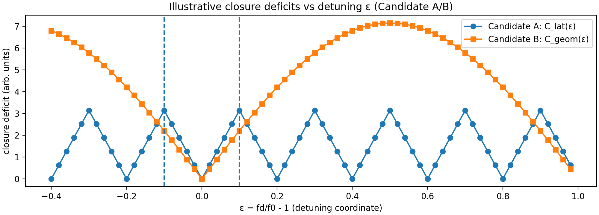
\[ C_{\text{geom}}(\tau_0;\varepsilon)=2\rho(\tau_0)\,|\sin(\pi\varepsilon)|,\qquad \rho(\tau_0)=R+a\cos\tau_0. \]

This metric is implemented in the simulation code as an illustrative bridge between detuning and observable mismatch.

---

6. Minimal perturbation model and basin boundary intuition

Introduce a scalar detuning coordinate \(\varepsilon\), which in the simulation is operationally:

\[ \varepsilon=\frac{f_d}{f_0}-1. \]

6.1 Candidate A under small perturbations (harmonic restoration + basin boundary estimate)

Let \(\Delta_0\) be exactly closing: \(n\Delta_0=2\pi m_0\). Perturb along direction \(v\):

\[ \Delta(\varepsilon)=\Delta_0+\varepsilon v. \]

Then:

\[ C_{\text{lat}}(\varepsilon)=\min_{\ell\in\mathbb{Z}^4}\left\|n\varepsilon v-2\pi\ell\right\|. \]

For sufficiently small \(|\varepsilon|\), the minimum is at \(\ell^{*}=0\) and:

\[ C_{\text{lat}}(\varepsilon)\approx n\|v\|\,|\varepsilon|,\qquad V(\varepsilon)\approx \kappa n^2\|v\|^2\,\varepsilon^2. \]

A first basin boundary estimate occurs near:

\[ |\varepsilon|\sim \frac{\pi}{n\|v\|}, \]

which the simulation prints as an illustrative “basin boundary estimate.”

6.2 Candidate B under detuning (smooth mismatch)

With \(\varepsilon\) interpreted as a small per-cycle angle mismatch, we obtain:

\[ C_{\text{geom}}(\tau_0;\varepsilon)\approx 2\pi(R+a\cos\tau_0)\,|\varepsilon|. \]

---

7. Definitions

CCR (Closure-Compatible Resonance). Resonant organization that remains compatible with a closure constraint; resonance is “useful” only if it keeps trajectories inside (or returning to) admissible basins. Closure deficit \(C\). Nonnegative scalar functional with \(C=0\) on the admissible set. Candidate A \(C_{\text{lat}}\). \(C_{\text{lat}}(\Delta)=\min_{m\in\mathbb{Z}^4}\|n\Delta-2\pi m\|\) (quantized closure basins). Candidate B \(C_{\text{geom}}\). \(C_{\text{geom}}(\tau_0;\varepsilon)=2(R+a\cos\tau_0)|\sin(\pi\varepsilon)|\) (observable mismatch model). AG (Admissibility Gradient). \(\mathbf{F}_{\mathrm{AG}}=-\nabla V\) with \(V\approx \kappa C^2\). PAC (Phase-Aligned Control). Phase-aware perturbations that bias dynamics into admissible basins at minimal energy, rather than brute suppression. Operational entrainment closure on \(S^1\). \(C_{\text{phase}}=1-\mathrm{PLV}\), where: \[ \mathrm{PLV}=\left|\frac{1}{N}\sum_k e^{i2\pi f_d t_k}\right| \]

over event times \(t_k\) [1].

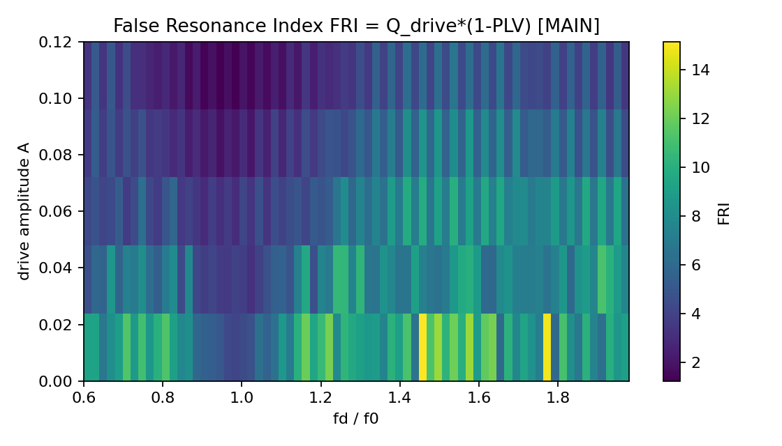
False resonance. Drive-like spectral signature without closure improvement: elevated near-drive spectral sharpness while \(C_{\text{phase}}\) remains high (PLV low).

---

8. Phase-Aligned Control (PAC): stabilize by biasing, not suppressing

Synchronization/locking phenomena commonly produce amplitude–detuning “tongue” regions (Arnold tongues), where sufficient coupling/authority yields phase locking [2]. The Kuramoto model is a canonical paradigm for how phase interactions organize into synchronized states [6]; PAC adopts this spirit but replaces “synchronization = success” with “closure-compatible synchronization = success” [7].

8.1 Closure-qualified control objective

A closure-qualified control objective can be posed as minimizing a closure-aware cost:

\[ J(p)=\alpha\,C_{\text{phase}}(p)+\beta\,\Pi_{\text{intermittency}}(p)+\gamma\,\Pi_{\text{false-res}}(p), \]

where \(p\) are control parameters (e.g., amplitude \(A\), frequency \(f_d\), phase offsets, spatial phasing), \(\Pi_{\text{intermittency}}\) penalizes burstiness (e.g., CV, kurtosis), and \(\Pi_{\text{false-res}}\) penalizes “spectral sharpness without closure.”

8.2 Plasma exemplars (pattern, not exhaustive review)

• RMP ELM control: modest, spectrally tuned perturbations can reorganize edge transport and modify ELM behavior in multiple machines, motivating a phase/structure lens rather than brute suppression [3].
• Phase synchronization between control system and plasma: phase-coherent feedback has been discussed as a distinct synchronization mechanism in plasma control contexts [4].

These examples motivate PAC as a control hypothesis: phase-aligned interventions can bias dynamics into more admissible coherent regimes.

---

9. Proxy simulation: “plasmoid reconnection entrainment” as an intermittency/locking testbed

This section presents a minimal intermittent system designed to test closure-qualified control logic. It is a minimal intermittent system designed to validate the control logic: closure-qualified entrainment, authority thresholds, detuning sensitivity, and false-resonance detection.

9.1 Model summary and the meaning of refractory

The simulator generates a bursty reconnection-rate proxy \(R(t)\) from threshold-triggered events and an exponential decay kernel. A refractory time prevents immediate retriggering; this represents a generic recovery/reset timescale (e.g., local relaxation, resource depletion, or reset dynamics) rather than a specific Sweet–Parker or plasmoid-instability timescale. The goal is to model “gated intermittency” where event timing jitter competes with a periodic control signal.

9.2 Drive coupling modes

The drive can couple in three modes:

• threshold modulation (default): no direct injection; the drive lowers/raises the burst threshold (“opens/closes the gate”)
• parametric: drive modulates the loading parameter \(a\)
• additive: drive injects directly into the internal variable

9.3 Operational closure metric and near-drive sharpness

Event times \(t_k\) define phases \(\phi_k=(2\pi f_d t_k)\bmod 2\pi\). The code computes:

\[ \mathrm{PLV}=\left|\frac{1}{N}\sum_k e^{i\phi_k}\right|,\qquad C_{\text{phase}}=1-\mathrm{PLV}. \]

For driven systems, “Q” is computed meaningfully near the drive frequency \(f_d\) (not at the global PSD peak): the script computes a local peak in a window around \(f_d\) and defines \(Q_{\text{drive}}=f_{\text{peak}}/\mathrm{BW}_{1/2}\) using a half-power bandwidth. Baseline \(f_0\) is estimated from the global PSD peak (appropriate for intrinsic frequency estimation).

9.4 MAIN/ROBUST sweeps and the authority threshold

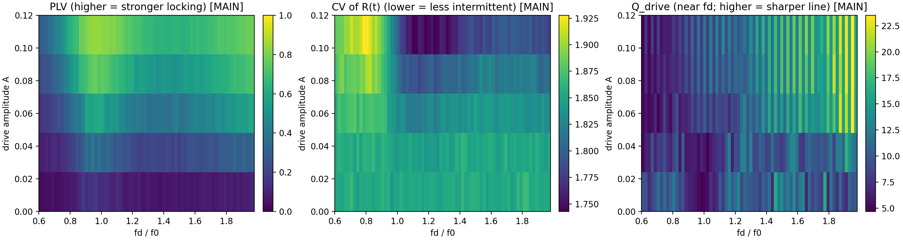
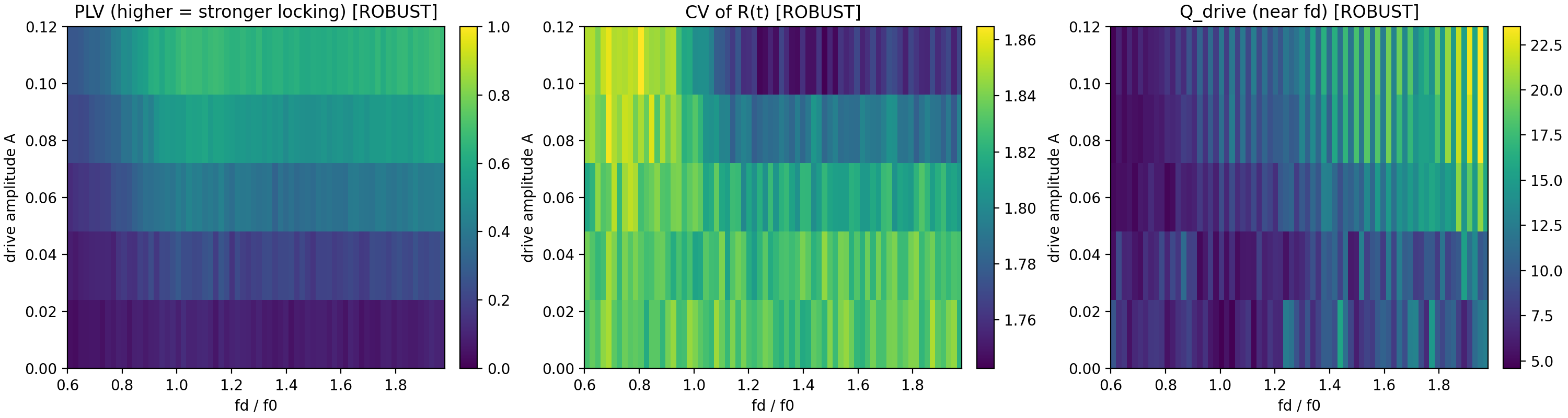
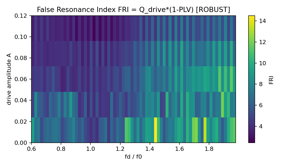
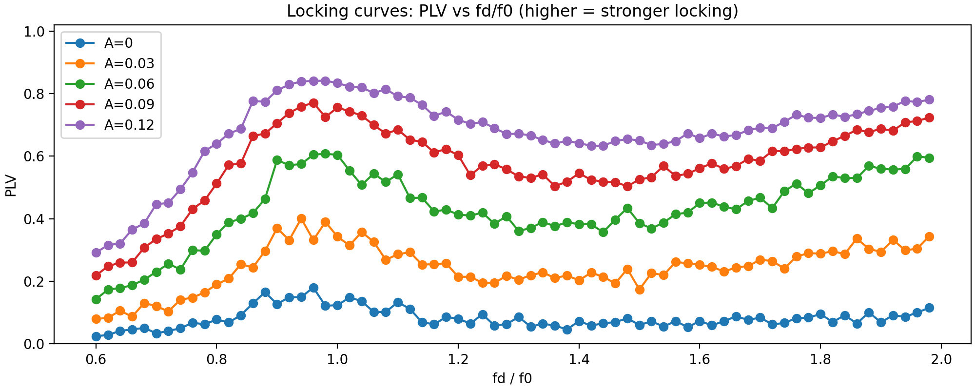
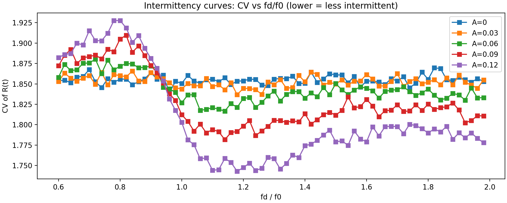
The script runs a MAIN sweep and a ROBUST sweep (higher noise) over amplitude \(A\) and ratio \(f_d/f_0\), aggregating over \(n_{\text{rep}}\) random seeds per grid cell. Heatmaps are saved for PLV, CV, and \(Q_{\text{drive}}\), plus “locking curves” (PLV vs \(f_d/f_0\) for each \(A\)).

Key result: a clear locking region appears only above a minimum \(A\). This is consistent with a burst-gated system: the drive must have enough authority to overcome event timing jitter to produce strong closure. The script prints tongue widths for PLV≥0.8. This qualitative behavior matches classic locking-region intuition (Arnold tongues) but here the “coupling strength” corresponds to control authority in a stochastic gated process [2]. Statistical note (recommended reporting): because PLV depends on stochastic event timing and event counts, a robust presentation should report per-cell uncertainty (std or bootstrap CI) for PLV/\(C_{\text{phase}}\), and typical event counts per grid cell. The current code stores only means; extending it to also save std/CI would strengthen the evidence section.

9.5 One-off comparisons: baseline vs resonant vs off-resonant vs broadband

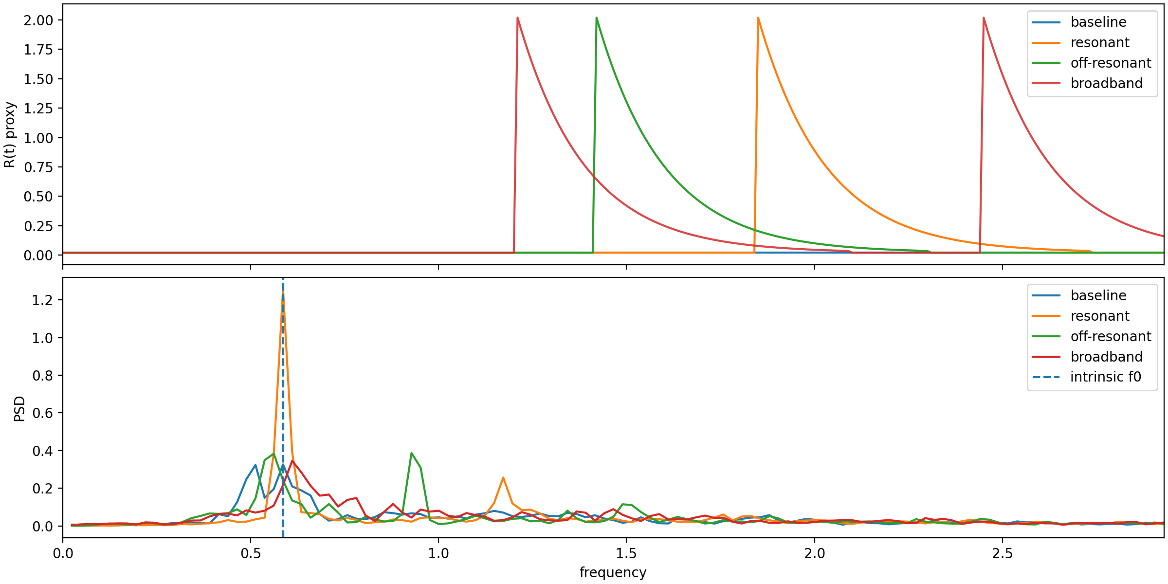
The script runs a one-off block and prints summary statistics, global PSD peak (baseline), and PLV/\(C_{\text{phase}}\)/\(Q_{\text{drive}}\) for driven cases.

From the reported sample run:

Condition	PLV	\(C_{\text{phase}}\)	\(Q_{\text{drive}}\)	Interpretation
Baseline (repeated)	-	-	-	estimates intrinsic \(f_0\), intermittency baseline
Resonant drive (\(A=0.09\), \(f_d\approx f_0\))	0.785597	0.214403	12	stronger closure (lower \(C_{\text{phase}}\))
Off-resonant (\(A=0.09\), \(f_d=1.6f_0\))	0.611291	0.388709	12.6667	partial coherence, worse closure
Broadband (\(A=0.09\))	0.118388	0.881612	6.25	activity without closure (anti-PAC)

Drive power in this table is not equal across rows. The amplitude parameter \(A\) is not a power. The sine drive is \(A\sin(2\pi f_d t)\), of mean square \(A^2/2\); the broadband drive is normalized to unit variance and then scaled by \(A\), of mean square \(A^2\). At the common setting \(A=0.09\) the broadband row therefore receives twice the drive power of the two sinusoidal rows (0.0081 against 0.00405). The comparison is not like-for-like, and the asymmetry runs against the broadband case: it is the row that received more power and produced the worst closure. Comparisons intended to be power-matched should scale the sinusoidal amplitude by \(\sqrt{2}\). What this supports:

• Detuning sensitivity: closure is best near \(f_d/f_0\approx 1\).
• Alignment > energy: broadband drive can increase activity (events) while destroying closure, and does so here while receiving twice the power.
• False resonance: off-resonant can show high near-drive sharpness without commensurate closure, hence “spectral sharpness ≠ closure” and the need to optimize \(C_{\text{phase}}\), not just \(Q_{\text{drive}}\).

This is the operational motivation for CCR/PAC: avoid interpreting “a sharp line near the drive” as success unless closure improves.

9.6 Candidate A/B deficits vs detuning: explicitly didactic

The script plots Candidate A \(C_{\text{lat}}(\varepsilon)\) and Candidate B \(C_{\text{geom}}(\varepsilon)\) versus detuning \(\varepsilon\), including an illustrative Candidate-A basin boundary estimate. These curves are didactic closure landscapes generated from the analytical definitions; they are not fitted or inferred from the burst simulation data. Their purpose is to connect “quantized basin vs smooth mismatch” pictures to the detuning coordinate used in sweeps.

9.7 Reproducibility checklist

For reproducibility of the proxy simulations, the following are explicitly specified:

• parameter ranges for \(A\) and \(f_d/f_0\);
• number of repetitions \(n_{\text{rep}}\) per grid cell and random seed handling;
• method for estimating intrinsic frequency \(f_0\) (global PSD peak);
• definition of near-drive spectral sharpness window for \(Q_{\text{drive}}\);
• typical event counts per run and their variability.

All numerical results shown are generated from the single-file script listed in Appendix B with no hidden state.

---

10. Discussion: integration, risks, and falsifiable hooks

10.1 What this paper supports

• A clean derivation path: closure deficit \(\to\) penalty \(\to\) admissibility gradient yields generic harmonic restoration near closure.
• Two complementary deficit constructions: quantized basin (Candidate A) and observable mismatch (Candidate B).
• An operational closure metric on \(S^1\): \(C_{\text{phase}}=1-\mathrm{PLV}\), tied to standard synchronization literature [1].
• In an intermittent gated system, locking requires authority, and spectral sharpness near the drive is not equivalent to closure.

10.2 Falsifiable hooks (general + plasma)

General driven systems (beyond plasmas): In intermittently bursting or thresholded oscillators (stick–slip, relaxation oscillators, spiking neurons, Q-switched lasers), one can observe “false resonance”: increasing near-drive spectral sharpness without improving event-phase closure. PAC predicts explicitly optimizing \(C_{\text{phase}}\) yields lower-energy stabilization than optimizing spectral criteria alone. This aligns with cautions that spectral coherence measures can mislead about true phase locking [5]. Plasma/control contexts: Phase-coherent control/plasma synchronization mechanisms have been discussed as distinct from brute suppression; CCR/PAC frames these as biasing into admissible closure regimes rather than “overpowering” instabilities [4].

10.3 Remaining limitations (explicit)

• The choice of \(\mathbb{T}^4\) is a constructive modeling choice; future work can test whether fewer/more phases are needed for particular applications.
• The proxy simulation would benefit from uncertainty reporting (PLV std/CI per cell), parameter sensitivity (noise, refractory), and multi-mode extensions. §10.4 now reports bootstrap intervals and a null arm; the §9 sweeps do not.
• The efficiency target is not invariant to the operating point (§10.4.1). Inter-event-interval CV is drive-independent, which is what the comparison requires, but any drive that raises the mean loading rate lowers it without organizing anything. Under coupling that does work on the state, a steady bias consequently beats phase-coherent drive and the §10.4 kill criterion fails.
• The phase-scrambled arm is not spectrum-matched (§10.4). It matches center frequency and power only, and no stronger match is available, since coherence time and bandwidth are conjugate. Phase structure and spectral concentration are therefore not separated by this comparison.
• The admissibility score cannot order admissible configurations (§3.3). Choosing among available locks requires the primitive period, which the \(V(C)\) machinery does not carry.
• The closure principle is regime-dependent (§1.1). Its validity here rests on the driven dissipative setting, and the framework's structural papers operate in a regime where the sign is reversed.
• \(C_{\text{phase}}\) is defined relative to the drive frequency \(f_d\). It is a measure of approach to a chosen lock, not a drive-independent measure of organization, and it should not be used as the target state in an efficiency comparison between drives of different spectral character. §10.4 specifies a drive-independent alternative.
• No prediction unique to this framework has yet been demonstrated. The locking phenomenology reported here (authority thresholds, tongue-like regions, spectral sharpness decoupled from phase locking) is consistent with standard synchronization theory [2,6], and so is the coherence-time dependence measured in §10.4. CCR supplies a control objective and a bookkeeping for it; it has not yet produced a measurement that standard synchronization analysis would not also predict. What §10.4 settles is narrower but not nothing: it fixes the direction and the size of the cost advantage, and rules out the reading that narrowband forcing alone accounts for it.

10.4 The efficiency claim, measured

Section 1 asserts that phase-aligned interventions stabilize at lower energetic cost than brute suppression. As reported in §9.5 that claim is evidenced in the quality at fixed amplitude direction. The operationally decisive form is the inverse:

> Fix a target state defined without reference to the drive. Compare the minimum input energy required to reach it under different drive protocols at matched power.

Protocol:

1. Target. Choose an organization metric that makes no reference to \(f_d\), for example the coefficient of variation of the inter-event interval, or any equivalent regularity measure of the event train. Fix a threshold on it.

2. Cost. Define input energy as \(E=\int \! d(t)^2\,dt\) over the drive signal \(d(t)\), and match this quantity, not the amplitude parameter, across protocols (§9.5).

3. Arms. At minimum: phase-coherent drive at the intrinsic event frequency; phase-scrambled drive at the same center frequency and the same power; broadband; and a steady (DC) bias.

4. Report \(\eta = E_{\text{incoherent}}/E_{\text{coherent}}\) at the fixed target.

Kill criteria, stated in advance. If the coherent arm does not reach the target at materially lower energy than the broadband and DC arms, the efficiency claim fails and PAC has no cost advantage to offer. More sharply: if the coherent arm does not also beat the phase-scrambled arm, which is matched in center frequency and in power, then the effect is attributable to narrowband forcing alone, the result reduces to classical resonance, and nothing in the closure framing is doing work. That second comparison is the one that carries the claim.

The scrambled arm is matched in center frequency and in mean square, not in realized spectrum, and versions of this paper through v1.2.1 described it as spectrum-matched in error. Measured on the generator at the reported settings, the coherent drive places all of its power within \(\pm 5\%\) of \(f_0\) while the scrambled drive places 0.20 to 0.22 there and 0.48 to 0.54 within \(\pm 15\%\). No stronger matching is available in this comparison: coherence time and bandwidth are conjugate, so a drive whose phase is randomized on a timescale \(\tau_c\) necessarily carries bandwidth of order \(1/\tau_c\). What the arm therefore isolates is coherence at fixed center frequency and fixed power, which is what the companion \(\tau_c\) prediction below measures directly. Separating phase structure from spectral concentration requires a different control, two signals sharing a magnitude spectrum and differing in phase, and is not attempted here.

A companion prediction, should the first survive: effectiveness at fixed power and fixed center frequency should depend monotonically on the coherence time of the drive, with the transition located near the system's own event-recurrence timescale.

Result, and a correction to how it was inferred. The criteria above were fixed before the first run; an earlier pilot informed the choice of metric and amplitude range but is not a run quoted here. Simulation release v1.1.0 implements the protocol as --efficiency and --coherence, at 12 repetitions per cell, and versions v1.2.0 and v1.2.1 of this paper reported it against a no-drive baseline of 0.178: a coherent minimum of 0.0036, off-resonant at 21.8×, and phase-scrambled, broadband and DC not reached beyond 34×. That inference rule was defective and is superseded here. It fixed the target at 90% of a single undriven realization, then compared it against driven runs at other seeds and recorded the first power level to dip below. Between-seed spread in the undriven baseline is 0.191 ± 0.016 over 400 realizations, the same order as the 10% effect being detected, and the rule requires no crossing to persist. Substituting an arm carrying no drive at all, the rule reports the target reached in 3 of 40 baseline seeds. The v1.2.0 figures remain reproducible as outputs of that rule and are not withdrawn as such, but the rule does not support them.

Simulation release v1.2.0 adds --efficiency-paired and leaves --efficiency unchanged, so the superseded numbers stay reproducible. It changes three things:

1. Paired baseline. Every driven run is divided by an undriven run at its own seed, so the target is a 10% reduction against that realization's own baseline rather than against a separate draw.

2. Sustained crossing. A crossing counts only if the arm holds the target across two consecutive swept powers. The run is required to be local rather than to extend to the top of the sweep, because the coherent arm is non-monotone: it loses the target at high power, where over-driving destroys regularity. A rule demanding persistence to the sweep limit inverts the comparison, disqualifying the coherent arm and admitting an off-resonant arm that only crosses in the final two cells.

3. Uncertainty, and a permanent null arm. The crossing power is bootstrapped over seeds, and an undriven run is carried through the identical pipeline as a control.

At 24 seeds and 2000 bootstrap resamples, against a mean undriven ISI CV of 0.191 ± 0.013:

Drive arm	Minimum power to reach target	Relative to coherent	95% CI	Never reached
Phase-coherent at \(f_0\)	0.00202	1×	[0.00202, 0.0036]	0%
Off-resonant (\(1.6 f_0\))	0.0784	38.7×	[0.0784, 0.0784]	0%
Phase-scrambled at \(f_0\)	not reached	> 60×	—	98.6%
Broadband	not reached	> 60×	—	100%
Steady (DC) bias	not reached	> 60×	—	99.0%
Null (no drive)	not reached	> 60×	—	100%

"Never reached" is the share of bootstrap resamples in which the arm does not reach the target anywhere in the swept range.

The correction moves the result toward the claim rather than against it. The off-resonant minimum does not move at all; what changes is the coherent minimum, which falls from 0.0036 to 0.00202 once the baseline noise masking it is removed, so the ratio grows. The coherent crossing is unchanged whether a crossing is required to persist for one, two or three consecutive powers. The null arm returns a ratio of exactly 1.000 ± 0.000 at every power, which is the property the superseded rule lacked.

The phase-scrambled arm is the one that carries the claim: matched in center frequency and in power, it fails to reach the target anywhere in the swept range in 98.6% of resamples, so the advantage is not attributable to narrowband forcing alone. Its closest approach is 0.939 ± 0.021 of baseline against a target of 0.90. Broadband drive makes regularity monotonically worse, reaching 2.08× baseline at the top of the sweep. DC drive is flat, between 0.92 and 1.01 of baseline throughout, and never reaches the target in the gating configuration used here; §10.4.1 records that this does not hold when the drive is coupled so as to do work on the state.

The companion prediction also holds. At fixed power (0.0100) and fixed center frequency, ISI CV falls monotonically with drive coherence time \(\tau_c\): 0.215 at \(\tau_c=0.3\)s, 0.186 at 3s, 0.150 at 7s, 0.110 at 30s, against 0.109 for a pure sine. The transition sits near \(\tau_c \approx 3\text{–}16\) times the mean inter-event interval of 1.87s, and at short coherence the drive leaves the system less regular than no drive at all. This rules out the reading that the scrambled arm merely had too short a scramble period: the dependence is a continuum in \(\tau_c\), not a threshold artifact.

What this does not establish. The model is a gated relaxation-oscillator proxy, not MHD, and carries no magnetic field, helicity, or Taylor state. The result shows that in a system relaxing through intermittent events, drive coherence buys organization that drive power cannot. Whether that transfers to plasma is unmeasured; §10.2 names the experimental setting where it could be tested.

#### 10.4.1 Dissipation, coupling, and where the criterion fails

Two objections to the result above concern the physics of the model rather than the statistics: that such a ratio comes free in a system without losses, and that it depends on how the drive is coupled. The first does not apply. The second does, and it bounds the claim.

Dissipation. The state variable carries a linear leak \(-bx\) at \(b = 0.75\ \mathrm{s^{-1}}\), giving \(\tau_{\mathrm{relax}} = 1.33\) s against a mean inter-event interval of 1.87 s, so it decays faster than the system fires. Every event resets it to \(x = 0\), so no amplitude accumulates across cycles, and a 0.25 s refractory gate follows each event. This is the opposite of a high-quality-factor resonator, and the accumulation mechanism that would make the ratio free is unavailable for a stronger reason: in the threshold coupling used above, the drive does not appear in the state equation at all. The update is \(dx = (a - bx)dt + \sigma\sqrt{dt}\,\xi_t\), identical with the drive on or off, and the drive enters only as \(\theta_{\mathrm{eff}} = \theta(1 - d(t))\). It gates when the system may fire rather than pushing on what accumulates, so \(E = \int d(t)^2 dt\) is a control-effort functional and not work delivered to the state. Coupling, and a failure of the kill criterion. Because the argument above turns on the drive doing no work, the result must be checked where it does. In additive coupling the drive enters the state equation directly. Under the same paired protocol, extended power grid, 24 seeds:

Drive arm	Minimum power to reach target	Relative to coherent
Steady (DC) bias	0.0064	0.22×
Phase-coherent at \(f_0\)	0.0289	1×
Off-resonant, phase-scrambled, broadband	not reached	> 78×

A steady bias reaches the target 4.5 times more cheaply than coherent drive, which fails the kill criterion stated above, and the result reported in §10.4 is therefore specific to gated coupling rather than general. The mechanism is not mysterious and it indicts the target metric: a constant additive drive raises the loading rate, steepening the ramp to threshold, so first-passage dispersion falls without anything being organized. Across the swept range the DC arm takes the event count from 106 undriven to 417, while the coherent arm moves it only to 134. Inter-event-interval CV is drive-independent, which is the property §10.3 requires of it, but it is not invariant to the operating point, and any drive that raises mean loading will lower it. The oscillatory arms remain unreachable in this coupling, so the comparison among timed drives survives; the comparison against an untimed bias does not.

Note also that additive and parametric coupling coincide at the default \(a = 1.0\), where both add \(d(t)\,dt\) to the state, so they do not constitute independent checks.

---

11. Conclusion

At the common amplitude setting \(A=0.09\), resonant drive achieves PLV = 0.786 while broadband achieves 0.118, a 6.6× difference. The two are not matched in energy: as set out in §9.5, the broadband case receives twice the drive power. The result is therefore that the higher-energy drive produced the weaker closure, which strengthens the direction of the claim while making the headline figure a comparison at equal amplitude, not at equal energy.

Off-resonant shows higher spectral sharpness than resonant (\(Q_{\text{drive}}\) 12.67 vs 12.00) but worse closure (\(C_{\text{phase}}\) 0.389 vs 0.214). Optimizing for spectral sharpness selects the wrong target.

Alignment determines efficiency more than amplitude. Stated carefully: within this proxy, at drive powers differing by a factor of two in the wrong direction, alignment still dominated the outcome. The properly power-matched form of that comparison is measured in §10.4: reaching a fixed, drive-independent target costs 38.7× less under phase-coherent drive than off-resonant, and phase-scrambled, broadband and steady drive do not reach it at all in the gating configuration. Two limits are equally part of the result. Under coupling that does work on the state, a steady bias reaches the target more cheaply than coherent drive and the pre-registered kill criterion fails (§10.4.1). And nothing measured here is unique to this framework (§10.3).

This motivates the closure-first framework:

• CCR: stability corresponds to closure-compatible resonance
• AG: closure penalties produce restoring gradients
• PAC: phase-aligned perturbations bias dynamics into admissible basins

---

Appendix A. Notation and core definitions

• \(Q\): configuration space; \(A\subset Q\): admissible set.
• \(C(q)\): closure deficit, \(C=0\iff q\in A\).
• \(V(C)\): closure penalty; locally \(V\approx \kappa C^2\).
• \(\mathbf{F}_{\mathrm{AG}}=-\nabla V\): admissibility gradient.
• \(f_0\): intrinsic peak frequency (baseline global PSD peak).
• \(f_d\): drive frequency; \(r=f_d/f_0\); \(\varepsilon=r-1\).
• \(\mathrm{PLV}\), \(C_{\text{phase}}=1-\mathrm{PLV}\) computed from event times.
• \(Q_{\text{drive}}\): near-drive spectral sharpness computed around \(f_d\).

---

Appendix B. Simulation reproducibility and artifacts

Code artifact: plasmoid_entrainment_sim-v1.2.0.py (single-file runnable module), simulation release v1.2.0. The superseded v1.1.0 is retained so the figures it produced stay reproducible. See also the reproduction notes and requirements.txt. Dependencies: numpy, scipy, matplotlib.

The simulation artifact is versioned independently of this paper. Figures 1-8 and every sweep result in §9 are reproduced unchanged by simulation release v1.0.0. Release v1.1.0 adds the §10.4 instrumentation without altering any v1.0.0 output: a drive-independent target metric (inter-event-interval CV), explicit energy accounting with exact power matching across drive shapes, and phase-scrambled and steady-bias drive modes. Release v1.2.0 adds the paired-baseline inference protocol described in §10.4 as --efficiency-paired, and leaves --efficiency and every earlier output unchanged, so the superseded v1.2.0-paper figures remain reproducible alongside the corrected ones. Note that the drive amplitude parameter \(A\) is not a power (§9.5).

Reproduce the current §10.4 table with

```

python plasmoid_entrainment_sim-v1.2.0.py --efficiency-paired

```

the §10.4.1 coupling check with --efficiency-paired --drive-mode additive --eff-rms 0.02,0.05,0.08,0.12,0.17,0.24,0.32,0.45,0.60,0.80,1.10,1.50, the companion coherence-time prediction with --coherence, and the superseded v1.1.0 result with --efficiency. Each writes a JSON record of every cell; the paired runs take a few minutes because they carry an undriven partner per seed and 2000 bootstrap resamples.

Core parameters exposed by CLI: drive mode (threshold, parametric, additive), refractory time, amplitude list, ratio list, noise levels, number of replications \(n_{\text{rep}}\), and one-off comparison controls. Saved artifacts (by default):

• sweeps.npz containing grids and MAIN/ROBUST metric maps plus didactic Candidate A/B arrays.
• oneoff_timeseries.npz storing time series and event times for baseline/resonant/off-resonant/broadband comparisons.

Saved figures (intended placement: Section 10 below):

• heatmaps_main.png: PLV, CV, \(Q_{\text{drive}}\) on MAIN sweep.
• heatmaps_robust.png: same under higher noise.
• locking_curves_plv.png: PLV vs \(f_d/f_0\) curves per \(A\).
• intermittency_curves_cv.png: CV vs \(f_d/f_0\) curves per \(A\).
• timeseries_psd.png: time series overlays + PSD comparisons for one-offs.
• candidateA_B_deficits.png: didactic Candidate A/B vs \(\varepsilon\).

---

Appendix C. Quantum numbers as closure invariants (optional interpretive lens)

This appendix provides an optional interpretive extension. It offers a compact interpretation: conserved “quantum numbers” can be viewed as invariants labeling inequivalent closure classes (winding, holonomy, non-abelian closure), and confinement can be framed as a non-closure constraint on isolated components. The intent is to guide intuition about admissible structure, not to replace Standard Model dynamics.

---

12. Figures (simulation outputs)

---

Revision history

v1.3.0. Corrects §10.4 following independent review. The measured direction and the conclusions are unchanged; the inference rule behind the numbers was defective, and one pre-registered criterion is now recorded as failing.

• The §10.4 inference rule is superseded. It set the target at 90% of a single undriven realization, compared it against driven runs at other seeds, and took the first power level to dip below. Between-seed baseline spread (0.191 ± 0.016 over 400 realizations) is of the same order as the 10% effect, and no crossing had to persist. An arm carrying no drive at all reaches the target under that rule in 3 of 40 baseline seeds. Simulation release v1.2.0 adds a paired baseline, a sustained-crossing requirement, bootstrap intervals, and a permanent null arm.
• The corrected numbers are larger, not smaller. The off-resonant minimum is unchanged at 0.0784. The coherent minimum falls from 0.0036 to 0.00202 once baseline noise masking it is removed, so the reported ratio moves from 21.8× to 38.7×, and the arms that do not reach the target now carry a bootstrap share rather than a single observation. The null arm returns exactly 1.000 at every power.
• Added §10.4.1, and one kill criterion now fails. The dissipation inventory and the fact that the drive does no work on the state in the gating configuration are stated explicitly. Under coupling that does do work, a steady bias reaches the target 4.5× more cheaply than phase-coherent drive, which fails the criterion stated in §10.4 and makes the headline result specific to gated coupling. The cause is a defect in the target metric: inter-event-interval CV is drive-independent but not invariant to the operating point.
• Corrected the description of the phase-scrambled arm. v1.1.0 through v1.2.1 called it matched in spectrum and power. It matches center frequency and power only, placing 0.20 to 0.22 of its power within ±5% of \(f_0\) against 1.00 for the coherent arm. No stronger match is available, because coherence time and bandwidth are conjugate.
• §10.3, §11 and Appendix B updated accordingly. §11 no longer describes the efficiency measurement as an open item.

v1.2.1. Appendices A-C were marked at title level rather than section level, so they were absent from the generated table of contents. Heading level corrected; no text changed. v1.2.0. Runs the §10.4 test rather than only specifying it.

• §10.4 reports the equal-target energy comparison. Reaching a 10% reduction in inter-event-interval CV costs 0.0036 in drive power under phase-coherent drive and 0.0784 off-resonant; phase-scrambled, broadband and steady-bias drive do not reach it anywhere in the swept range, beyond 34x the coherent cost. The companion coherence-time prediction is also confirmed and rules out a scramble-period artifact. (The inference rule behind these figures is superseded in v1.3.0.)
• §10.3 and Appendix B updated accordingly. The claim that no prediction unique to the framework has been demonstrated still stands: the measured behaviour is consistent with standard synchronization theory.
• Requires simulation release v1.1.0, which adds the instrumentation and leaves all v1.0.0 output unchanged. The code is now published alongside the paper and linked from Appendix B, so §10.4 can be re-run independently.

v1.1.0. Corrections following internal review. No figure, sweep, or numerical result is changed, and the simulation artifact is unchanged at release v1.0.0.

• Added §1.1. The closure-first principle is not regime-neutral, and every claim in this paper is a driven dissipative claim. In v1.0.0 the justification for CCR was inherited from the non-dynamical closure language of Paper I and read as though admissibility implied persistence generally; under conservative perturbation the sign is reversed. The conclusions are unaffected because the systems treated here are forced, damped and intermittent, but the derivation path is now stated correctly.
• Extended §3.3. An admissibility score built from the closure deficit alone cannot rank admissible configurations against one another, because the deficit vanishes identically on the admissible set while robustness there varies by orders of magnitude with the primitive period.
• Corrected §9.5 and §11. The one-off comparisons are matched in the amplitude parameter \(A\), not in drive energy. The sine drive has mean square \(A^2/2\) and the broadband drive \(A^2\), so at \(A=0.09\) the broadband case receives twice the drive power. The direction of the reported result is unaffected, and the asymmetry runs against the broadband case: it received more power and produced the worst closure. The v1.0.0 phrase "identical energy input" was incorrect.
• Added §10.4, restating the efficiency claim as a pre-registered test with kill criteria stated in advance, including a phase-scrambled drive arm described there as matched in both spectrum and power (corrected in v1.3.0: center frequency and power only). Added four limitations to §10.3, including that \(C_{\text{phase}}\) is drive-referenced and that no prediction unique to this framework has yet been demonstrated.
• Appendix B now pins the simulation artifact version and notes the instrumentation §10.4 requires.
• Completed the reference list. Entries [1]-[5] carried only a title, venue and link in v1.0.0, with no author or year; they now give full bibliographic detail, as do the companion-paper entries.
• Corrected citation numbering in §8 and §10.2. Reference [4] was never cited while claims belonging to it cited [5], and the spectral-coherence caution cited [6] instead of [5]. The Kuramoto attribution in §8 now cites [6] directly.
• Typographic fix in §5.1 and §6.1: the superscript asterisk in \(m^{}\) and \(\ell^{}\) was written with an invalid escape, which failed to typeset and displayed as raw source in the web rendering of v1.0.0. Notation and meaning are unchanged.
• Typographic fixes in the abstract and in §1, §2 and §9.5, where parenthetical dashes had been flattened to hyphens ("performance-especially", "closure-internal", "closure-hence"). Wording is otherwise unchanged.

v1.0.0. Initial preprint.

---

References

1. Aydore, S., Pantazis, D., & Leahy, R. M., A note on the phase locking value and its properties. NeuroImage 74, 231–244 (2013).

2. Schilder, F. & Peckham, B. B., Computing Arnol′d tongue scenarios. J. Comput. Phys. 220, 932–951 (2007).

3. Fenstermacher, M. E. et al., ELM control by resonant magnetic perturbations: overview of research by the PEP ITPA group. 23rd IAEA Fusion Energy Conference, Daejon (2010).

4. Chapman, S. C., Lang, P. T., Dendy, R. O., Giannone, L., & Watkins, N. W., Control system-plasma synchronization and naturally occurring edge localized modes in a tokamak. Phys. Plasmas 25, 062511 (2018).

5. Lowet, E., Roberts, M. J., Bonizzi, P., Karel, J., & De Weerd, P., Quantifying neural oscillatory synchronization: a comparison between spectral coherence and phase-locking value approaches. PLOS ONE 11, e0146443 (2016).

6. Acebrón, J. A. et al., The Kuramoto model: A simple paradigm for synchronization phenomena. Rev. Mod. Phys. 77, 137–185 (2005).

7. Jakovels, E., ResonanT⁴: Modular Closure and Transverse Geometry. resonant4.io (2026). doi:10.5281/zenodo.18157442.

8. Kolmogorov, A. N., On the conservation of conditionally periodic motions under small perturbation of the Hamiltonian. Dokl. Akad. Nauk SSSR 98, 527–530 (1954).

9. Arnold, V. I., Proof of a theorem of A. N. Kolmogorov on the invariance of quasi-periodic motions under small perturbations of the Hamiltonian. Russian Math. Surveys 18, 9–36 (1963).

10. Greene, J. M., A method for determining a stochastic transition. J. Math. Phys. 20, 1183–1201 (1979).

11. Arnold, V. I., Small denominators I: mappings of the circumference onto itself. Amer. Math. Soc. Transl. 46, 213–284 (1965).

12. Jakovels, E., Quantum Numbers as Closure Invariants. resonant4.io (2026). doi:10.5281/zenodo.18157869.